Transactions on Machine Learning Research (TMLR), 2026
Generalizing Beyond Suboptimality: Offline Reinforcement Learning Learns Effective Scheduling through Random Solutions

CDQAC (Conservative Discrete Quantile Actor-Critic) is an offline reinforcement learning (offline RL) method for the job shop scheduling problem (JSP) and the flexible job shop scheduling problem (FJSP). It learns a dispatching policy from a fixed dataset of existing schedules, without interacting with a simulator during training, and it learns best when those schedules were made by picking actions at random.
Trained only on random solutions, CDQAC reaches an average gap of 10.7% with greedy decoding and 5.9% with sampling on the FJSP evaluation sets. That is better than when it is trained on dispatching-rule or genetic-algorithm data, and better than every other offline method tested. It needs only 10 to 25 training instances.
Abstract
Online reinforcement learning (RL) approaches have demonstrated strong performance on Job Shop Scheduling (JSP) and Flexible JSP (FJSP) problems by learning scheduling policies through direct interaction with simulated environments. However, these methods often require extensive training interactions, limiting their sample efficiency and practical applicability. Motivated by this challenge, we introduce Conservative Discrete Quantile Actor-Critic (CDQAC), an offline RL algorithm that learns effective scheduling policies directly from static, suboptimal datasets. CDQAC couples a quantile-based critic with delayed policy updates to estimate the return distribution of machine–operation pairs. Extensive experiments on JSP and FJSP benchmarks demonstrate that CDQAC consistently outperforms the data-generating heuristics, surpasses state-of-the-art offline and online RL baselines, and is highly sample efficient, requiring only 1 to 5% of the original dataset to learn high-quality policies. Our analysis suggests that, in scheduling, offline RL performance is governed mainly by state–action coverage rather than the quality of individual trajectories. Scheduling couples a dense reward aligned with the makespan objective with equal-length trajectories across heuristics, enabling effective learning from a broad range of behaviors. Consistent with this observation, datasets generated by a simple random heuristic with broader coverage let it outperform policies trained on datasets produced by stronger heuristics such as Genetic Algorithms.
Offline RL for scheduling, without a simulator or expert data
Online reinforcement learning methods for job shop scheduling, such as L2D and DANIEL, learn by interacting with a simulated shop floor, often for millions of steps. That is slow, and a simulator rarely captures every detail of a real factory.
Offline RL learns from a fixed dataset instead, for example the schedules a plant has already run. Because it learns what each decision is worth rather than copying the decisions it sees, it can end up better than the data it was trained on. Our earlier method, Offline-LD, showed that this works for JSP, but it relied on near-optimal solutions from a constraint programming solver, which are expensive to produce and intractable for large instances. CDQAC drops that requirement: it learns strong policies for both JSP and FJSP from suboptimal data, down to schedules made at random.
How CDQAC works
CDQAC builds a schedule one decision at a time. At every step it looks at the partial schedule and picks a machine–operation pair: which operation runs next, and on which machine. The reward for a step is the negative increase in the partial makespan, so the rewards of a finished schedule add up to exactly minus its makespan.
Conservative Q-learning keeps unseen actions in check
An offline agent never sees what happens after actions that are missing from its dataset, so a naive critic can overestimate them and the policy will chase those errors. CDQAC adds a Conservative Q-Learning (CQL) penalty that pushes down the value of pairs outside the data.

A quantile critic for every machine–operation pair
A Dual Attention Network (DAN) encoder, adapted from DANIEL, embeds the operations and machines. On top of it, the critic predicts a distribution over returns, as a set of quantiles in the style of QR-DQN, for each candidate pair instead of a single value. It uses a dueling design with separate inputs: the value stream sees a global embedding of the schedule, and the advantage stream sees the operation, machine and pair embeddings. That split suits scheduling, where the number of candidate pairs changes at every step.

Delayed policy updates
The actor, which is the scheduling policy itself, is updated only once every η critic updates. This stops errors in the bootstrapped critic from compounding into the policy. In the ablation study this is the component that matters most, and it matters more on larger instances with larger action spaces.
Why random data works: coverage beats quality
On standard offline RL benchmarks, expert data beats random data. In scheduling we found the opposite, and traced it to two structural properties:
- A dense reward aligned with the objective. Every decision receives a reward that is a calibrated share of the final makespan, so even a bad schedule tells the critic what each of its steps cost.
- Equal-length trajectories. Every heuristic, good or bad, makes exactly one decision per operation, so all trajectories for an instance have the same length and none is favored for being shorter.
With both properties in place, what limits offline RL is state–action coverage: how many different situations and decisions the data contains. A random policy maximizes coverage by construction.
State–action coverage of each training dataset, relative to the dispatching-rule dataset
The paper tests this explanation directly. Breaking either property, by cutting episodes short or by switching to a sparse or proxy reward, hurts the random dataset the most.
Results on job shop and flexible job shop benchmarks
Flexible job shop (FJSP): the weakest data gives the best policy
We trained CDQAC and five other offline methods (behavior cloning, IQL, TD3-AWR and two Offline-LD variants) on four datasets, each produced by a different heuristic: priority dispatching rules (PDR), a genetic algorithm (GA), both combined, or uniformly random decisions. Averaged over all FJSP evaluation sets, CDQAC beats every other method on every dataset, and its best result comes from the random data, even though the random heuristic itself is by far the weakest.
Average gap on the FJSP evaluation sets, by training dataset
- Data-generating heuristic (best)
- CDQAC, greedy
- CDQAC, sampling
| Training data | Heuristic (best) | CDQAC, greedy | CDQAC, sampling | Best other, greedy |
|---|---|---|---|---|
| Random | 28.16 | 10.68 | 5.86 | 14.72 (TD3-AWR) |
| PDR | 14.13 | 12.34 | 6.57 | 18.63 (TD3-AWR) |
| GA | 6.74 | 13.06 | 6.43 | 13.91 (BC) |
| PDR + GA | 6.74 | 11.31 | 5.87 | 15.29 (TD3-AWR) |
Against online reinforcement learning
CDQAC trained on random data also surpasses the state-of-the-art online RL baselines on the FJSP and JSP benchmarks, including DANIEL, the online method whose encoder it builds on. On the Taillard JSP benchmark:
| Method | Type | Greedy | Sampling |
|---|---|---|---|
| MWR | dispatching rule | 19.4 | – |
| MOR | dispatching rule | 19.9 | – |
| L2D | online RL | 27.3 | – |
| Offline-LD | offline RL | 25.6 | – |
| DANIEL | online RL | 18.2 | 14.4 |
| Residual | online RL | 17.0 | 14.6 |
| CDQAC (random data) | offline RL | 15.2 | 11.7 |
Mean gap (%) on the Taillard benchmark, lower is better. For reference, exact MIP and CP solvers with a 30-minute limit per instance reach 8.4% and 2.0%. CDQAC was trained on the random 10×5 dataset. The paper also compares further JSP-specific methods.
What each component contributes
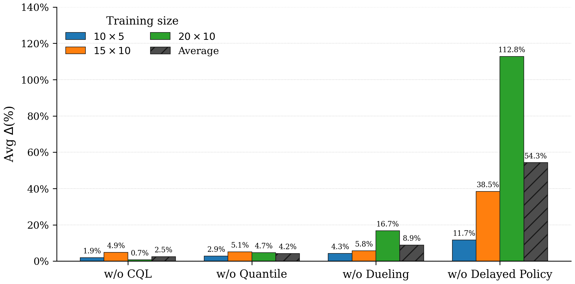
Removing the delayed policy update hurts most: the gap grows by 54.3% on average, and by 112.8% when training on 20×10 instances. The dueling architecture shows the same pattern at a smaller scale (8.9% on average, 16.7% on 20×10), while removing the quantile critic or the CQL penalty costs 4.2% and 2.5% on average.
Sample efficiency
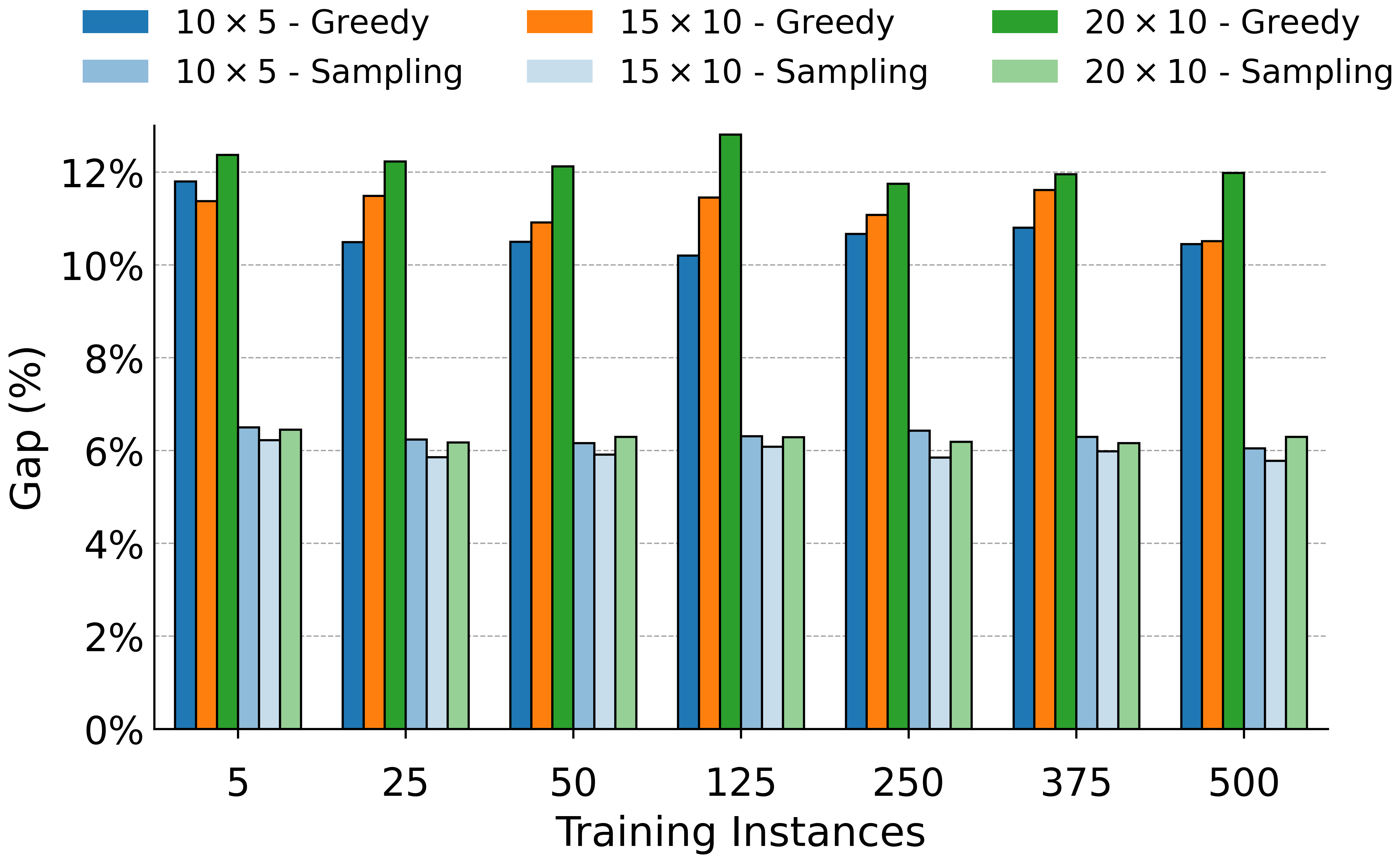
CDQAC reaches competitive performance with 10 to 25 training instances, typically 1 to 5% of the data that online RL baselines train on. Dataset size barely matters: from 5 to 500 random training instances, the gap on the Brandimarte and Hurink FJSP benchmarks stays around 6% with sampling and moves by at most about one and a half percentage points with greedy decoding.
Code, datasets and pretrained checkpoints
Everything needed to reproduce the paper is public. The code on GitHub (MIT license) trains CDQAC and the offline baselines (behavior cloning, IQL, TD3-AWR and both Offline-LD variants) from a single entry point. The datasets and checkpoints on Hugging Face hold the JSP and FJSP training data from every heuristic (dispatching rules, genetic algorithm, random and ε-greedy dispatching rules), the evaluation instances, and pretrained policies.
git clone https://github.com/jesserem/CDQAC_scheduling
cd CDQAC_scheduling
pip install -r requirements.txt
python download_datasets.py eval checkpoints

# Evaluate a pretrained CDQAC policy (trained on random FJSP data, 10×5)
python eval_model.py checkpoints/fjsp/cdqac/cdqac_random_10_5.pt --eval_folder ./data/SD1/10x5
Frequently asked questions
What is offline reinforcement learning for scheduling?
It trains a scheduling policy from a fixed dataset of past decisions instead of from trial and error in a simulator. The dataset can be historical schedules or solutions from existing heuristics. Unlike imitation learning, offline RL learns how valuable each decision is, so the policy can outperform the schedules it learned from.
Can offline RL learn from random or suboptimal schedules?
Yes. Trained on uniformly random solutions, CDQAC reaches a 5.9% average gap on the FJSP evaluation sets with sampling, its best result across the four training datasets, ahead of data from a genetic algorithm.
Why does random data beat genetic-algorithm data here?
Scheduling has a dense reward tied to the makespan and trajectories of equal length, so coverage, not quality, is the bottleneck. Random solutions contain 7.7 times as many unique state–action pairs as dispatching-rule solutions, against 2.96 times for the genetic algorithm, which gives the critic more to learn from.
How much training data does CDQAC need?
Competitive performance takes 10 to 25 training instances, typically 1 to 5% of the data online RL methods train on.
Does CDQAC need a simulator or expert solutions?
Not for training. It learns from a static dataset and does not need solutions from an exact solver. In the paper the datasets come from simple heuristics; in practice they could come from historical schedules.
How does CDQAC compare with online RL methods such as DANIEL or L2D?
Trained only on random data, CDQAC surpasses the online RL baselines in the paper. On the Taillard JSP benchmark its mean gap is 15.2% with greedy decoding, against 18.2% for DANIEL and 27.3% for L2D.
How is CDQAC different from Offline-LD?
Offline-LD (Machine Learning, 2025) was the first end-to-end offline RL method for JSP and learned from high-quality solutions produced by a constraint programming solver. CDQAC learns from low-quality data, handles both JSP and FJSP, and combines a quantile critic with a separate actor, a dueling design and delayed policy updates.
What are the limitations?
Training directly on large FJSP instances (20×10) becomes unstable as the action space grows. Policies trained on small instances generalize well to larger ones, and factorizing the action space into separate operation and machine choices is a promising way to scale further.
Cite this paper
@article{remmerden2026generalizing,
    title={Generalizing Beyond Suboptimality: Offline Reinforcement Learning Learns Effective Scheduling through Random Solutions},
    author={Jesse van Remmerden and Zaharah Bukhsh and Yingqian Zhang},
    journal={Transactions on Machine Learning Research},
    issn={2835-8856},
    year={2026},
    url={https://openreview.net/forum?id=4vVhm4817Q}
}Earlier arXiv versions of this paper were titled “Generalizing Beyond Suboptimality: Offline Reinforcement Learning Learns Effective Scheduling through Random Data”.
Related work
- Offline Reinforcement Learning for Learning to Dispatch for Job Shop Scheduling (Offline-LD). Our first offline RL method for JSP, trained on constraint programming solutions.
- Flexible Job Shop Scheduling via Dual Attention Network-Based Reinforcement Learning (DANIEL). Source of the DAN encoder and the FJSP environment.
- Job Shop Scheduling Benchmark: Environments and Instances for Learning and Non-learning Methods. Used to generate the genetic-algorithm datasets; code.